Organizing Chaos Part 2: Excelling at Story Timelines

One Spreadsheet to Rule Them All!

In Part One of Organizing Chaos, I shared my Microsoft Word Compendium with you. This week, I’m showing off my Microsoft Excel Timeline! Are you needing a well-organized timeline to track your storylines with? Then let the adventure unfurl…

AI art generated by Midjourney

Toolkit

I specifically use Microsoft Excel (Office 365 desktop edition). However, there are also free alternatives that can perform the same functions: Google Sheets (online) and LibreOffice (“Calc” desktop software)

Rationale for Excel

I turned to Excel for tracking my timelines for two simple reasons:

1. Sorting

2. Filtering

The Primordial Engine Excel Timeline

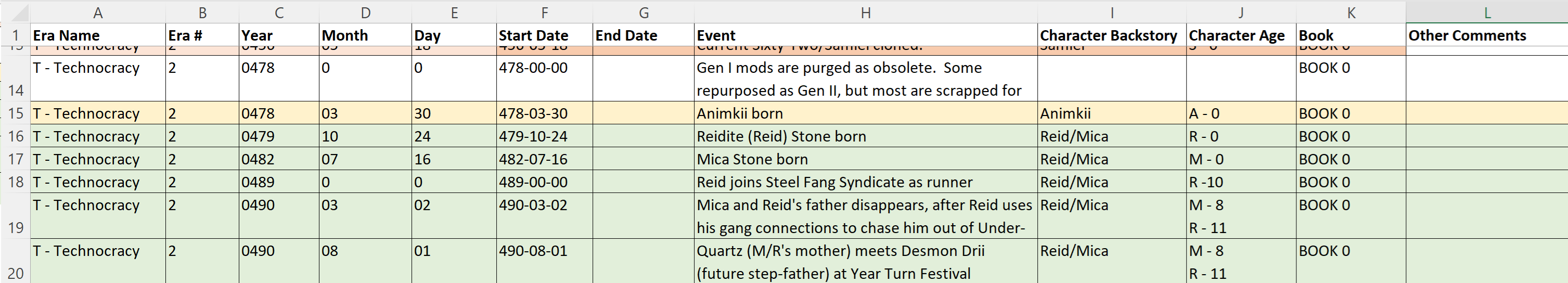
Behold, a short snapshot of my own series’ timeline spreadsheet to give you a taste of the journey you’re embarking on!

Create Your Own Excel Timeline

Basics

If you need a refresher on Excel basics, check out Microsoft’s Basic Tasks in Excel

Step 1: Create Spreadsheet

File > New > Blank workbook. File > Save > name your spreadsheet.

Step 2: Create Your Columns Headers / Freeze Top Row

1. Type out the names of your column headers in the worksheet’s top row of cells. HINT! When you pick header names, think about things you want to SORT or FILTER by. See below for a list of headers I used (top screenshot is how it looks in the worksheet; bottom screenshot explains what each of my headers means).

   

   

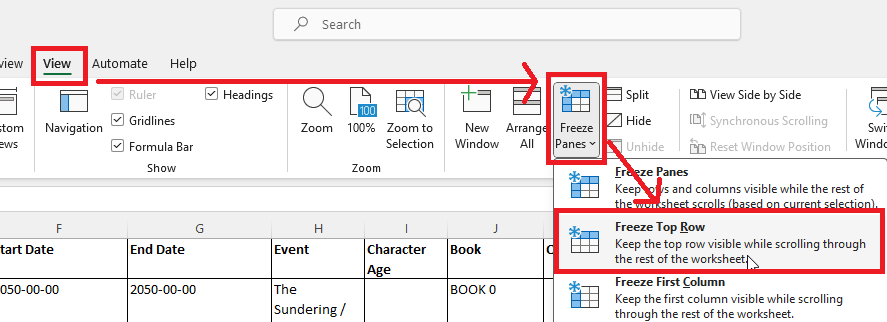
2. Freeze your top row so your headers are always visible. View > Freeze Panes > Freeze Top Row

   

Step 3: Dates

Standard Calendar / Dates

1. Add a “Dates” header name. Excel has built in Date formats that will recognize standard calendar dates.

2. If you don’t like how Excel displays your date (ie. it displays it as “Feb-05” instead of “February 5, 2023” then you can customize the date format.

Customizing Date Format

1. Highlight the cell(s) you want to format.

2. Right-click the highlighted cell(s) > Format Cells

3. In the Format Cells dialog box, select the Number tab, then select Date

4. In the Type list, you will see the predefined date formats. Choose one of these formats, or create a custom date format by clicking the Custom category (left pane).

5. Predefined date format: select the format from the list > OK button to apply the format. Creating Custom formats are outside the scope of this document, but here’s an in-depth document to guide you through it: Change Date Format Excel

6. The selected cell(s) will now display the date(s) in the customized format you specified.

Weirdo Calendars / Dates

Hello fantasy / sci-fi authors! If you have non-standard months / weeks that don’t match Excel’s predefined date formats, this section is meant for you!

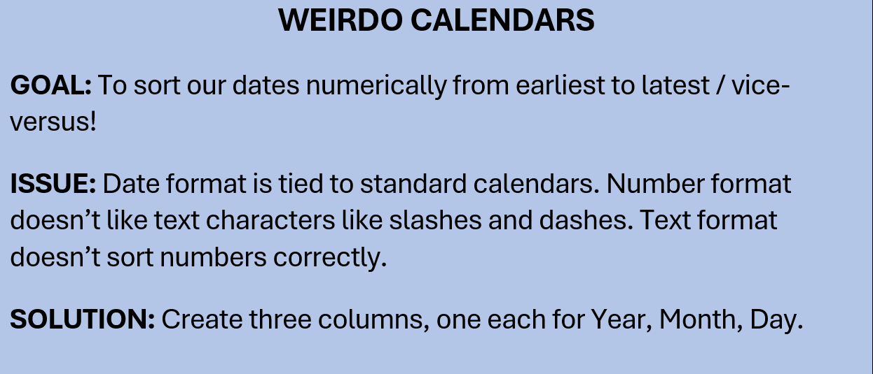
1. Insert three columns into your spreadsheet (right-click column > Insert). You need one each for Year, Month, Day.

2. (Optional) Display leading zeroes. By default, Excel will display 06 as 6, so if you want all your months to display the same number of digits, then you need to display leading zeros.

   1. Highlight the cell(s) where you want to display leading zeros.

   2. Right-click cell(s) > Format Cells

   3. In the Format Cells dialog box, select the Number tab, then select Custom.

   4. In the Type field on the right, enter the desired format for your numbers, including leading zeros. For example, if you want to display a 4-digit number with leading zeros, you use the format "0000" (four zeros).

   5. Click the OK button to apply the custom number format.

   6. Now, any number you enter in the selected cell(s) will display with leading zeros to match the format you specified.

3. Assign numbers to your dates. To make your weirdo calendar work, you will need to assign numbers to your years / months / days in the order you want them sorted. For example, in my future Earth, there is a 5-day floating week. It appears after the my twelfth month, so I assigned it the number 13 (for Month), even though it’s not a month, in order to make it sortable.

   

4. (Optional) Insert a Date column(s) for full date display. The three Year / Month / Date columns are useful for sorting, but you may still want an ‘at a glance’ display of the date. This will NOT be correctly sorted as it is not a standard date format—I also suggest formatting these Date columns as “text” (right-click cell > Format > Number tab > Text).

Step 4: Adding Other Columns

When adding new columns (right-click column > Insert), consider two things:

1. Do you want to sort by this column?

2. Do you want to filter by this column?

If you’re answer is YES to either question, then make sure the data added to sorted/filtered columns is consistent so it can be sorted/filtered correctly. For example, I make sure the spelling of character names in the Character Backstory is the same (I always use “Mica”, not “M” or “Mica Stone”).

Step 5: Fill Out Your Timeline

Fill in your timeline details.

Step 6: Extras

Borders

The gridlines you see by default in Excel are not borders. They exist as a guideline. If you want visible borders, you must explicitly define them.

1. Highlight the rows / columns in your sheet that you want to have borders.

2. On the Home tab, under the Format ribbon, click the Borders icon and select the type of border you want.

3. Your border will now be applied.

New Tabs / Worksheets

Each tab in an Excel workbook is called a worksheet. Use additional worksheets to track calendar details, holiday lists, and other information you don’t want on your main timeline worksheet.

1. To create a new worksheet, click the + sign beside your other tabs

   

2. To rename worksheet: right-click tab > Rename > type name

“Legend” Tab Example

“Calendars” Tab Example

Fill Cells with Color

Coloring cells can help you highlight important rows / columns (for example, I use it to mark out timelines tied to specific characters’ backstories)

1. Select the cell(s) to color > click the Fill bucket icon under Font ribbon > select the color

Sorting

Sorting in Excel lets you arrange data in a specific order based on the values in one or more columns of a worksheet. Use this to keep your dates in proper order.

Quick Sort (One Column)

1. Select a single cell in the column you want to sort.

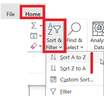
2. On the Home tab, in the Sort & Filter group, click Sort A to Z (earliest to latest) or Sort Z to A (latest to earliest)

Custom Sort (Multiple Columns)

Custom sorting by multiple columns in Excel allows further refinement of sorting order.

1. Select a single cell in any column.

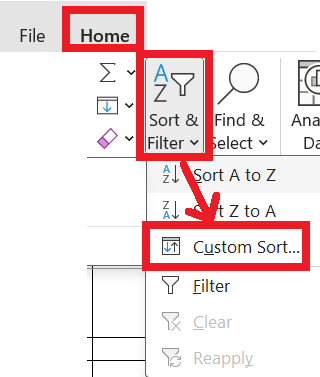
2. On the Home tab, in the Sort & Filter group, click Custom Sort

   

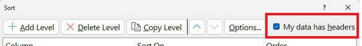
3. Check off “My data has headers”

   

4. Add the columns you want to sort by.

   1. Click Add Level to add new columns (to delete, select a column > click Delete Level)

   2. Leave Sort On at default of Cell Values.

   3. For Order, keep the order the same for all columns, unless you have a good reason.

   4. Arrange sorting levels. The columns are sorted from the order they appear in this list, from top to bottom (use up/down arrow buttons to move). In my own example, I have Era sorted first (to avoid mixing the dates between my two Eras). Next I sort by Year, Month, Day so that my dates will be sorted chronologically. If you are not using Weirdo Dates, you might have a single Date column which you can sort by instead.

      

5. Add non-date columns if required. Sometimes you want to subdivide dates by event types or characters involved. In these cases, you would place it above your highest date level (to show a list of dates for each character, I would place Character Backstory above Era because I have characters who have backstories crossing Eras).

6. Click OK

7. If you see the following error, select “Sort anything that looks like a number, as a number.” This will appear if you used Custom formatting for the cells (eg. leading zeroes) > OK

   

8. Your timeline is now sorted by date!

Filtering

Filtering in Excel allows you to display a subset of your data instead of the whole sheet. For instance, if I only want to see timelines associated with my character, Animkii, then I can use Filters to only show rows that have the Character Backstory of “Animkii”

1. Turn on the Filter: On the Home tab, in the Sort & Filter group, click Filter.

   

2. Once you turn on the filter, your top row / column headers will show drop-down arrows

   

3. On the column you want to filter by, click the drop-down arrow. You will see (Select All) and a list of your column’s contents. By default, (Select All) is selected, meaning all rows associated with this column are shown (unless filtered out by a different columns filter).

1. If you only want to see a few items listed, then uncheck (Select All) to clear all items. Then put check marks beside the ones you want to see. Click OK to apply the filter.

   

2. When a column is using a filter it will change the drop-down arrow to a funnel.

   

3. You can apply multiple column filters, but be aware that filters are cumulative. If I have Animkii filtered for Character Backstory, then I won’t be able to see any rows from Era 1, because none of her Character Backstory entries also belong to Era 1.

Turn Off Filters! (Great for Troubleshooting “Missing” Rows)

1. Remove Filter from one column:

   1. Click the filter drop-down arrow

   2. Put checkmark beside (Select All)

2. Turn off All Filters: On the Home tab, in the Sort & Filter group, click Filter (if it’s in use, the funnel icon will be outlined). Your header column filter drop-downs will disappear

   

Conclusion

In this week's post, we explored Microsoft Excel as a tool to construct a well-organized timeline for your fictional worlds, transforming your world-building chaos into a well-structured journey!